Do image file sizes get bigger as time goes on?

Lets start off with something simple and look at the cumulative file size. First we need to get the data

select file_size
from posts
order by post_id asc

And then make a graph.

file_sizes <- read.csv("ordered_file_size.csv")
png(filename="cumulative.png")
plot(
    cumsum(as.numeric(file_sizes[, 1])),
    main="Cumulative file size over time",
    type="l",
    xlab="Almost post_id (Time)",
    ylab="Total file size (Bytes)"
)

---

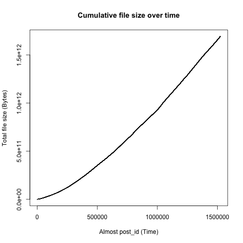
This doesn't look very useful. We do see that in the start posts were of a smaller file size, but we don't know much more than that.

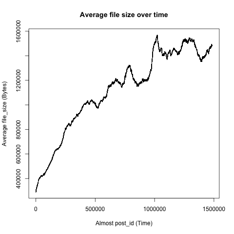
Well a next step could be to look at what the rolling average of file size was.

select 
    avg(file_size) over (
        order by post_id asc
        rows between 1 following and 1000 following
    )
from posts

Followed by

averages <- read.csv("rolling_avg.csv")
png(filename="rolling_avg_1.png")
plot(
    averages[, 1],
    main="Average file size over time",
    type="l",
    xlab="Almost post_id (Time)",
    ylab="Average file_size (Bytes)"
)

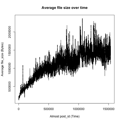
That looks pretty rough so lets increase the averaging range to 50000.